Bayesian Flow Networks (A Twitter Overview)

August 16, 2023

by Alex Graves, Rupesh Kumar Srivastava, Timothy Atkinson and Faustino Gomez

This post is a compilation of a Twitter thread introducing our paper on Bayesian Flow Networks. It gives a very high-level summary of the system in the paper.

We present a new perspective on the ideas related to diffusion models. BFNs combine Bayesian inference and neural nets to yield a model class with simple objectives that gracefully extends to discrete data.

We motivate BFNs from the perspective of compression (I’ll explain the figure below). The goal of learning is to minimize the cost of communicating the data, formally equivalent to fitting a probabilistic model with max. likelihood since the coding cost equals \(-\log(p_{model}(\text{data}))\).

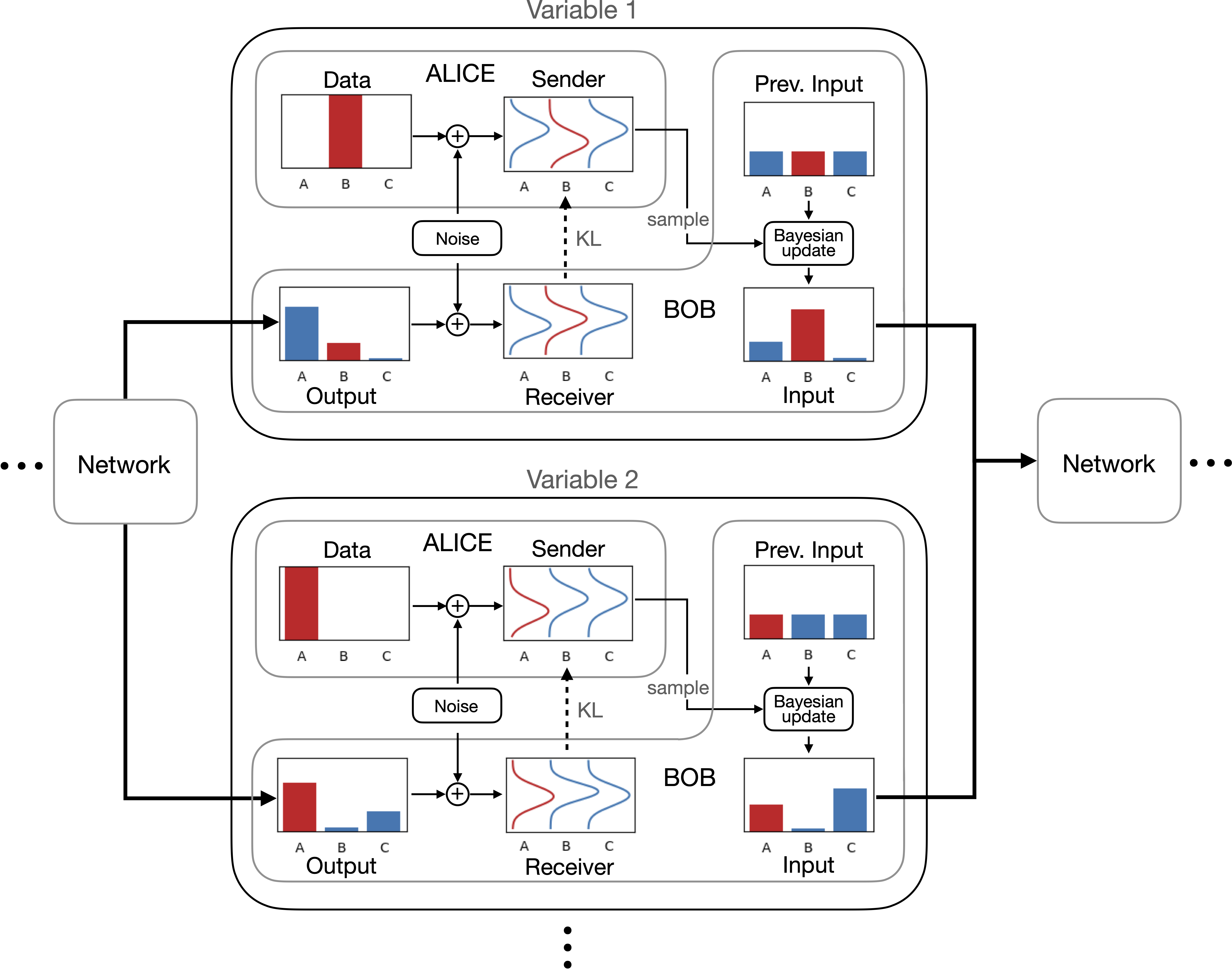
Warmup: Autoregressive models. Say Alice wants to transmit \(\mathbf{x}\) to Bob, \(\mathbf{x}\) has \(D\) variables or “tokens”, and both have access to the model. Alice sends token number \(d\) at step \(d\) encoded using the conditional model distribution at that step. The avg cost is the cross entropy in bits.

For training the model, we add up the costs at all \(D\) steps and minimize it. But what if instead of sending one token at a time, Alice sends a little information about all the \(D\) tokens at each step? Then Bob can decode all tokens in parallel, leading us to diffusion and BFNs.

Say Alice and Bob agreed on a noise distribution schedule: Alice will send a sample from \(\mathbf{x} + \text{noise}(t)\) at time \(t\). This “sender distribution” formalizes “a little information”. But which distribution to encode this sample with since Bob doesn’t know \(\mathbf{x}\)?

We need a “receiver distribution” that both Alice and Bob have access to, similar to autoregressive case, to encode/decode the noisy samples. Clearly, if Bob can guess \(\mathbf{x}\), guessing \(\mathbf{x} + \text{noise}(t)\) will follow, since \(\text{noise}(t)\) is known. Let’s focus on parameterizing that guess first.

Assume a simple factorized form for guessing \(\mathbf{x}\), e.g. a product of \(D\) normal distributions for continuous data, whose parameters \(\boldsymbol{\theta}\) (mean and variance) are initially unknown to Bob, so he starts with a prior (the standard normal).

We call the first guess above the “input distribution” \(p_{_I}\), because \(\mathbf{\theta}\) will be the inputs of our network. The output of the network \(\boldsymbol{\psi}\) will parameterize a similar, “output distribution” \(p_{_O}\). Both \(p_{_I}\) and \(p_{_O}\) will be updated at every step of the communication of noisy samples.

The Bayesian part is this: given previous \(\boldsymbol{\theta}\) and a noisy sample with known noise, we can compute new parameters \(\boldsymbol{\theta}'\) for certain distributions easily using Bayes’ theorem. This works because we are operating on independent distributions for each variable, so calculations are simple!

Putting it together:

• Create sender dist (Fig: A)
• Use input parameters \(\boldsymbol{\theta}\) to compute \(p_{_O}\) using the network (Fig: B)
• Use \(p_{_O}\) to construct a receiver dist and communicate a sample from the sender dist (Fig: C)
• Use Bayesian update to compute \(\boldsymbol{\theta}\) for the next step (Fig: D)

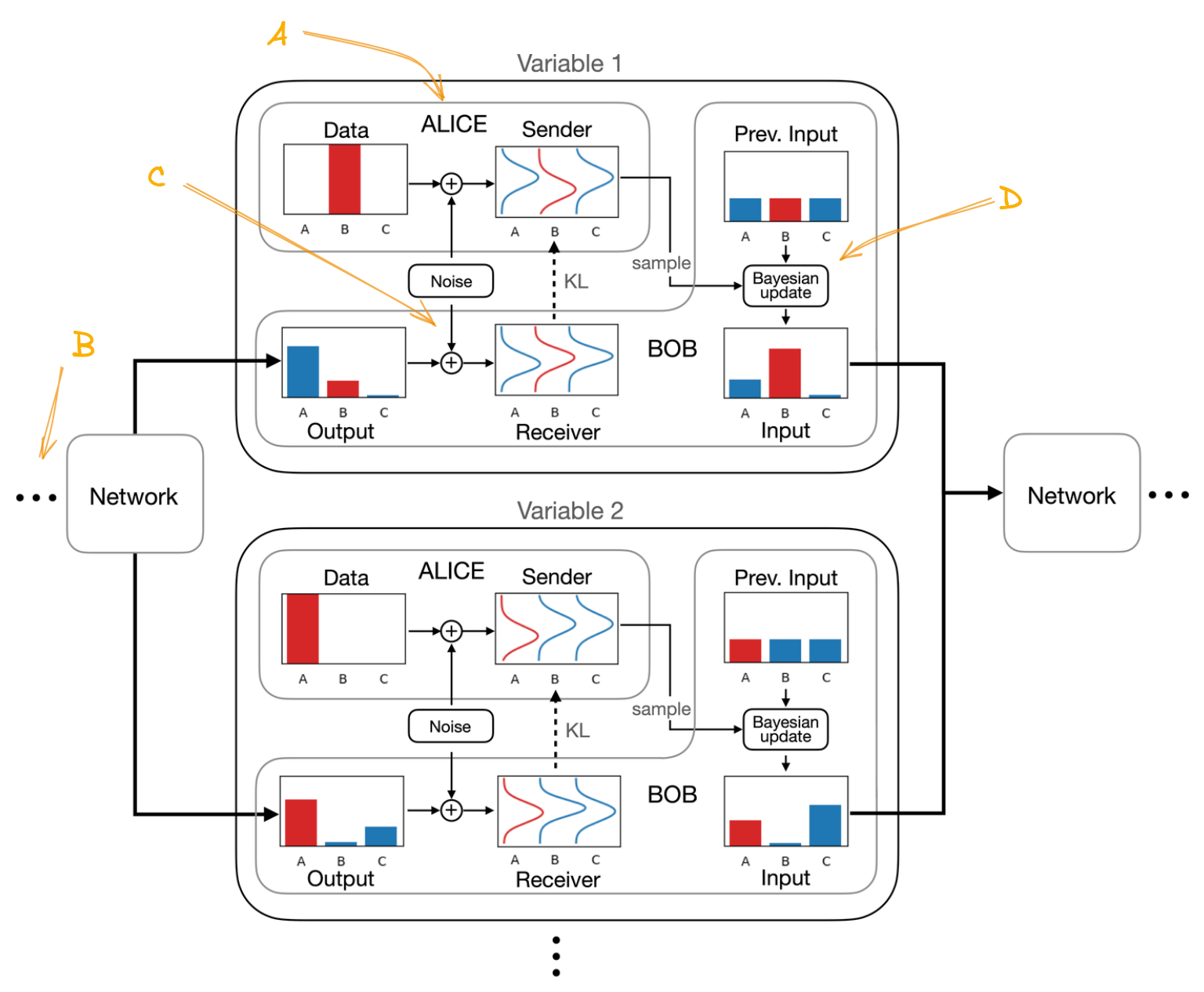
Both \(p_{_I}\) and \(p_{_O}\) get updated over time. Bayesian inference precisely updates beliefs about independent variables, and the network models the relationships between the variables. In the continuous time limit, the Bayesian updates become a Bayesian Flow of information from \(\mathbf{x}\) to \(\boldsymbol{\theta}\).

The total communication cost is the sum of costs at each step, which is simply the KL divergence between the sender and receiver distributions (plus a small residual cost at the end). We minimize this to train the network.

Note that unlike diffusion models 1) there is no need to define a forward process 2) the noisy sender distributions are independent so deriving the loss in closed form is simple 3) the net maps from distribution to distribution, not data to distribution.

All this makes it possible for us to easily adapt the BFN framework to continuous, discretized and discrete data in the paper by choosing appropriate distributions. We get very good results on modeling MNIST, CIFAR-10 and text8. Check it out!